How Predictive Policing Models Are Built (2026)

Predictive policing models are statistical systems trained mostly on historical crime reports and other agency records. They score where and when crimes are likely to be reported in the near future, and some score individuals for investigative attention. Knowing how predictive policing models are built matters because a model recommendation becomes a patrol assignment, and a patrol assignment generates the next round of data the model learns from.

I have read through the vendor training guides, contract records, randomized field trials and investigative reporting that are publicly available on these systems, and the pattern is consistent: the engineering is fairly ordinary, and the hard problems are everything around it.

Below is the build pipeline in plain language, followed by what the output actually means, how accuracy gets tested, and what oversight is missing in most deployments.

Table of Contents

• What predictive policing models do
• What data goes into a predictive policing model
• How predictive policing models are built from raw data
• What modeling methods are commonly used
• How a model turns data into a risk score
• How predictive policing models are built and tested for accuracy and bias
• What happens when a model is deployed
• What safeguards and oversight should exist
• Frequently Asked Questions
• What data are predictive policing models built from?
• Are predictive policing models accurate enough to use in police work?
• Can predictive policing models be biased?
• Does a predictive policing score prove that someone will commit a crime?
• How can communities oversee predictive policing systems?
• Conclusion

What predictive policing models do

A predictive policing model takes historical incident data and produces a ranked forecast of future incidents, usually by location and time window. Officers or analysts receive that forecast as a patrol suggestion or a dashboard alert. The model does not see the future; it extrapolates patterns from records of what was reported before.

It helps to separate three ideas that often get bundled together. Hot spots policing is an evidence-based practice where officers go to places where crimes cluster, based on analysis rather than instinct. Predictive policing adds a model that projects those clusters forward in time and prioritizes which boxes to visit today. Risk assessment scores individuals rather than places, estimating the likelihood that a named person will be arrested, fail to appear, or reoffend.

The distinction matters because the accuracy bar is different for each. A place-based model can be useful and still concentrate patrol in the same neighborhoods it has always concentrated patrol in. A person-based score carries a much higher risk of being treated as evidence when it is not evidence at all.

The practical build, in eight steps, looks like this:

1. Collect years of incident reports, calls for service, arrest records, and sometimes outside datasets such as weather, business listings, or consumer device alerts.
2. Clean the records, dropping duplicates, fixing garbled addresses, and resolving inconsistent offense and location fields.
3. Geocode every record into a grid, often cells of roughly 500 by 500 feet, a resolution described in the published training material of one of the best-known vendors.
4. Choose a time window, such as the next seven days, so that forecasts line up with how shifts actually get planned.
5. Engineer features: counts by offense type, recent versus historical rates, day and hour patterns, proximity to known anchor points, and distance to the current patrol route.
6. Define the label, which is the event the model is trying to predict. Reports of crime, arrests, or calls are all labels and each one means something different.
7. Train and validate the model on part of the history and score it against a held-out period to see whether it would have beaten a simpler baseline.
8. Deploy into a workflow, where the score becomes a task, an alert, or a recommendation, and then monitor what officers actually did with it.

Steps one through six are where most of the real behavior lives. A model is a function of its inputs and its label, so changing what counts as an incident changes what the model believes.

What data goes into a predictive policing model

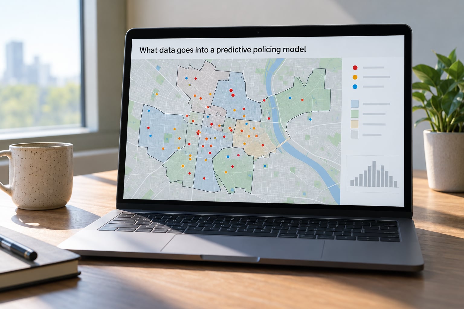
The typical input is agency data: reported incidents, calls for service from computer-aided dispatch, arrest records, traffic stops, warrant records, and sometimes body camera or GPS data from patrol vehicles. Departments that buy newer systems often add layers that were never part of the original academic literature, including neighborhood camera networks, alarm and sensor feeds, and commercial location or consumer data.

One investigation into how consumer camera alerts reached a major city’s police dashboards found officers receiving dozens of alerts in a single shift, with a substantial share describing non-criminal behavior such as a package left on a porch. That is a data ingestion problem before it is a policing problem: a feed that mixes trespass, curiosity and genuine emergencies produces a backlog nobody has time to triage.

Here is the split that residents usually find hardest to accept. Available data is whatever the department can obtain. Legitimate evidence is data that independently supports an investigative conclusion. The same arrest record is a fine training input and a poor basis for a stop, and plenty of systems blur that line because the pipeline treats all of it as columns in the same table.

Some also feed in non-police sources: risk terrain modeling overlays crime reports with land use features like bars, transit stops and vacant lots, on the theory that the environment generates opportunity. That approach is a different model from place-based prediction, and it should be evaluated on its own terms rather than as a variant.

How predictive policing models are built from raw data

Raw records arrive messy. The same address gets written four ways, one offense code covers everything from vandalism to assault, and a third of entries have no usable coordinates. Data engineers spend most of their time on this step, and every shortcut here quietly shapes the output.

Cleaning means deduplicating, normalizing addresses against a street database, standardizing offense categories, and deciding what to do with records that have no location. Geocoding then snaps each remaining point to the grid. A cell of roughly 500 by 500 feet holds a few city blocks, which is small enough to be useful for directed patrol and large enough to contain enough history to be statistically meaningful. Finer grids look impressive on a map and produce very noisy scores.

Feature engineering turns each cell into a vector of numbers. Typical features: incident counts in the cell over the last week, the same count over the last year, the share of violent versus property offenses, hour-of-day density, distance to the nearest recent incident, and counts from neighboring cells. Some systems include environmental variables such as proximity to a liquor license or a weather condition.

Labels come next, and this is the decision that quietly decides what the model means. A model trained on all reported incidents will rank cells with high call volume at the top. A model trained only on burglaries will ignore noisy calls entirely. A model trained on arrests inherits every difference in who gets stopped and who gets arrested, because arrest volume reflects enforcement as much as it reflects offending.

A worked example makes it concrete. Take one grid cell with nine incidents in the past year, two of them within the last week, both property offenses, both within 200 meters of a transit stop. Compare that to a nearby cell with four incidents in the past year and none recent. With a seven-day window, the first cell carries more weight on the recent-count feature and probably ranks higher. The score is a weighted sum of those numbers. Nothing in it is knowledge about the future; it is a smoothed echo of where reports already landed.

What modeling methods are commonly used

Most place-based systems start somewhere simple. Nearest-neighbor methods ask which cells historically produced similar patterns; kernel density estimation smooths incident points into a continuous probability surface. Bayesian methods such as the one behind a widely deployed vendor product combine recent incidents with a longer-run baseline through a time-decay term, so a busy cell fades if it goes quiet.

Logistic regression and gradient-boosted trees handle classification tasks, such as whether an incident will occur in a cell at all within the window. Time-series methods model hourly or weekly patterns separately from location. Clustering groups cells by profile so officers get a strategy rather than a single number. And a growing number of vendors now describe neural and foundation-model approaches that read text narratives of incidents, not just coordinates, to infer types and patterns that structured fields miss.

Public-sector teams often prefer something less flashy. When a score ends up in front of a city council, in a records request, or in a civil rights complaint, an interpretable model that produces a readable reason for each score is far easier to defend than a large ensemble nobody can explain. Some vendors will produce both, and the interpretable version is the one worth asking for.

How a model turns data into a risk score

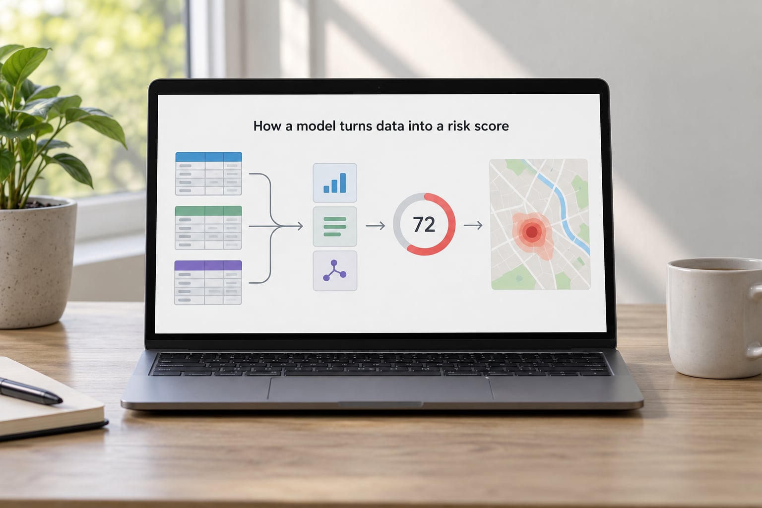
The mechanics are simpler than the marketing. A trained model stores a weight for each feature. The score is a weighted combination of the features, usually passed through a function that compresses the result between zero and one. A cell scoring high simply has a feature combination the model has learned to associate with incidents in the past.

Place-based outputs are scores for boxes and time windows. Person-based outputs are scores for named individuals, assembled from arrest history, prior contacts, associations in police records, and sometimes sealed records such as juvenile history. One well-known department’s person-scoring program assigned points for police contacts, then removed that feature after critics showed how the scoring reproduced the department’s own prior enforcement patterns.

Here is the line that should be stated plainly: a risk score is not a prediction that a particular person will commit an offense. It is a measurement of similarity to a profile built out of past records. In place-based systems, the score attaches to a location, not a resident. In person-based systems, it is a lead for investigative attention and nothing more, and treating it as anything more is how a weak signal becomes a stopped body.

How predictive policing models are built and tested for accuracy and bias

Evaluation is where most published claims get soft. The data is split chronologically rather than randomly, so the model is trained on the past and scored against a period it never saw, which is the only honest test for a forward-looking forecast. The model should then be compared against simple baselines, such as simply patrolling the cells with the highest historical counts. A complex model that cannot beat that baseline is not earning its complexity.

Error rates are reported in four ways. False positives are alerts for cells that stayed quiet, and in hotspot work they are arguably fine, because a wasted patrol hour has a low cost. False negatives are the serious category, since a predicted cell that stayed empty is a miss. Precision and recall summarize the tradeoff, and calibration answers a different question: when the model says 30 percent, does an incident actually land in that cell about 30 percent of the time.

Bias testing comes next, and it is mostly a measurement problem rather than a modeling one. Investigators compare alert rates, stop rates and arrest rates across neighborhoods and demographic groups. If the model flags areas that map onto previously patrolled areas, and patrolling creates records, the model is partly measuring its own past output. Research using a randomized controlled trial in Chicago, published in a peer-reviewed journal, tested whether a predictive patrol tool improved crime reduction over conventional patrol and found no improvement on the outcome that mattered, which is the sort of result that rarely appears in vendor marketing.

The ceiling nobody can lift is that these systems are evaluated against reported crime. Domestic violence, sexual assault, and most fraud go unreported. Where reporting depends on trust in police, the data understates crime most where a model is most confident, and any accuracy claim built on that data inherits the gap.

What happens when a model is deployed

Technical accuracy is not the same as operational accuracy. A model that improves forecast quality can still produce an alert list nobody can work through, and the real-world failure is usually a queue, not a score.

Integration is more work than vendors suggest. The forecast has to land somewhere an officer sees, attach to a task or a shift plan, and survive the fact that officers may ignore it. Practitioners inside departments often apply these recommendations selectively, which quietly breaks the feedback loop the vendor depends on and leaves the agency unable to evaluate the tool honestly. Monitoring usually means watching alert volume, response times and clearance rates, none of which measure crime reduction directly.

Retraining is another quiet hazard. Because the model’s inputs include its own downstream effects, a system retrained on recent data will learn from patrols it recommended itself. Departments that cancelled these programs, including Oakland, Richmond and Milpitas among the better documented cases, cited both ineffectiveness and profiling risk rather than a single defect.

Documentation usually stops at the vendor’s training manual, and that manual is often the most technical public document available, since it has to survive being obtained through a public records request.

What safeguards and oversight should exist

If a system is going to direct patrol resources, a reasonable baseline is not hard to write down. Independent audits should be able to reproduce the vendor’s headline accuracy claim, using the same data, without vendor cooperation on the analysis itself.

Public documentation should cover the data sources, the label definition, the validation results including baseline comparisons, and the known failure modes. Agencies should publish a plain-language summary alongside the technical material, and update it when the model is retrained.

Impact assessments belong before deployment rather than after a controversy, covering disparate impact, data collection practices, and whether the system expands rather than narrows police contact. Communities should have a formal route to influence procurement, and a city council vote should be required before a contract extends an existing deployment.

Two limits are worth writing directly into policy. A prediction should never be treated as probable cause or as independent evidence for a stop, a search, or a detention. And every dataset and score should carry an expiration date, because a score built on a person’s conduct years ago stops describing that person and starts describing the record-keeping habits of the department that made it.

Data minimization belongs in the same list. If a model does not need a field to work, the field should not be collected, and a score should expire when the underlying records age out. Appeals matter too: anyone subject to a person-based score should be able to see it, challenge it, and have an inaccurate record corrected.

Frequently Asked Questions

Conclusion

Building a predictive policing model is ordinary data work: collect records, clean them, snap them to a grid, engineer features, pick a label, train, validate against a baseline, and push the result into a shift plan. Every one of those steps makes a choice about what counts as evidence, and each choice carries into the score an officer sees.

So judge a system on five things: the quality and representativeness of its data, whether its validation beats a simple baseline, how much of the model is documented publicly, what safeguards and appeal rights exist, and what measurable change followed deployment. A claim about predictive power on its own tells you very little. If a city cannot answer those five questions about a system that already directs its patrols, that is the answer.