Trip planning algorithms find routes by turning a map into a weighted graph of roads and stops, then running a shortest-path search to find the lowest-cost connection between two points. When several stops are involved, a second layer sequences them, filters out anything that breaks a rule like opening hours, and re-weights the result as traffic changes.
That is the whole trick, and it is worth understanding before you trust a recommendation with a two-hour detour in it. Here is how each piece works, in the order the software actually does it.
Table of Contents
- How Trip Planning Algorithms Find Routes
- What Data Does a Trip Planning Algorithm Use?
- How Does a Route-Search Algorithm Compare Paths?
- How Algorithms Choose Between Fastest, Shortest, and Cheapest Routes
- How Live Traffic Data Changes the Recommended Route
- How Do Planners Rank Routes With Multiple Travel Modes?
- How Does a Trip Planner Account for Transfers and Schedules?
- Why Do Two Planners Suggest Different Routes?
- What Makes a Route Recommendation Useful in a Smart City?
- Frequently Asked Questions
- What algorithm is most commonly used to plan a trip?
- How does a trip planner use real-time traffic data?
- Does the shortest route always have the shortest travel time?
- How do transit planners find routes with transfers?
- Why might two trip planners recommend different routes?
- How often should a route be recalculated while traveling?
- Conclusion: Start With the Travel Objective
How Trip Planning Algorithms Find Routes
Every route planner, from a city transit app to a delivery fleet dispatcher, runs the same pipeline: build a graph, search it for the cheapest path, sequence the stops, filter what survives against real-world constraints, and re-weight the edges as conditions change. Each stage has different inputs and different failure modes.
- Load the network. Roads, rail lines, walking paths, ferry links and bike lanes become a graph of nodes and edges.
- Attach a cost to every edge. Travel time, distance, tolls, fuel use, gradient, footpath quality, or a blend weighted by the traveler’s preferences.
- Search the graph. A shortest-path algorithm such as Dijkstra or A* returns the cheapest path between two nodes.
- Sequence multiple stops. A routing heuristic decides the order the stops are visited in, since the order changes the total cost.
- Filter against constraints. Opening hours, reservation windows, vehicle capacity, driver hours and accessibility rules remove or reshuffle stops.
- Score the surviving options. Remaining routes are ranked on a multi-criteria score rather than a single number.
- Re-optimize as conditions change. Live traffic, missed connections and delays re-weight edges and trigger a fresh search mid-trip.
What Data Does a Trip Planning Algorithm Use?
Start with the network itself. OpenStreetMap supplies a surprising share of the base map for open planners, and transit agencies publish timetables in the GTFS format, which lists every trip, stop, arrival time and service frequency. Bikeshare and scooter systems publish vehicle positions through GBFS feeds.
On top of that sit the things that make a route real rather than theoretical: turn restrictions, one-way streets, bridge weight limits, tolls, seasonal closures, and speed limits per road segment. Add the observation layer and you have probe speeds from phones, loop detectors and buses reporting their own delay.
Then come the user inputs, which matter more than people expect. A wheelchair user, a traveler with a dog, a commuter avoiding tolls and a family of five with a daily driving limit are all different cost functions over the same graph. A planner that ignores your preferences is not broken, it is just answering a different question.
How Does a Route-Search Algorithm Compare Paths?
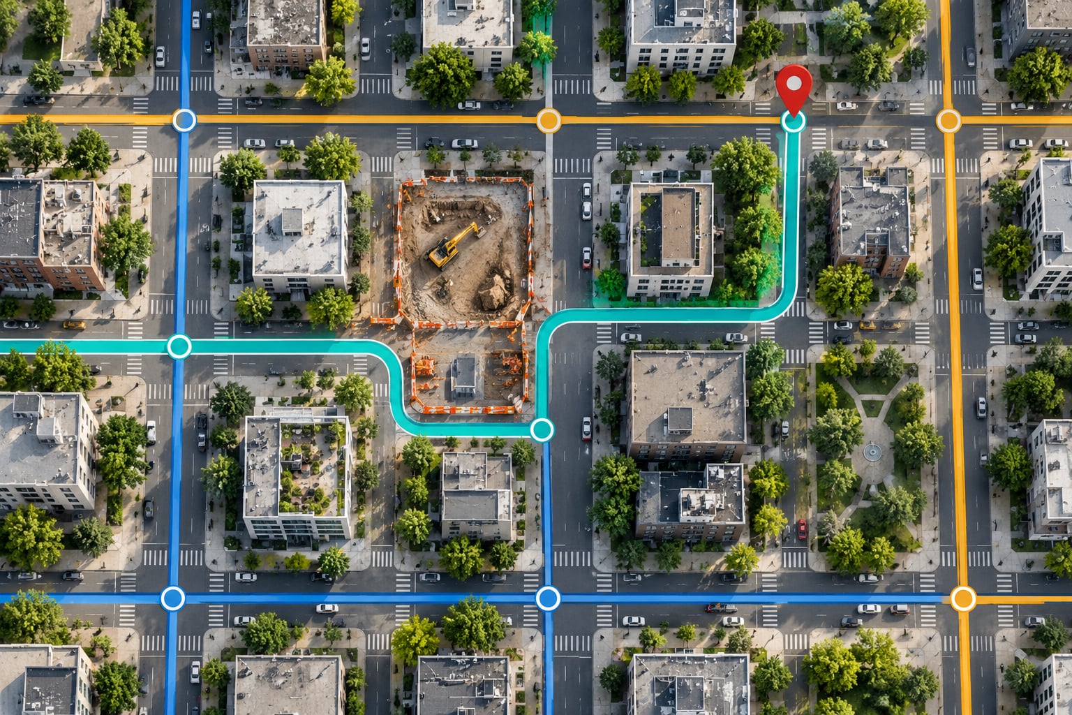
The road network is modeled as a weighted graph: intersections are nodes, road segments are edges, and every edge carries a cost. A shortest-path search then explores that graph without ever building the full list of possible routes.
Dijkstra’s algorithm works outward from your origin in widening rings of cost. It maintains a frontier of nodes it has reached, always expanding the cheapest one first. Once it pulls the destination off the frontier, no cheaper path can exist, because every other unexplored route already costs at least as much.
A* improves on that by adding a heuristic: an estimate of the remaining cost from a node to the destination, usually straight-line distance scaled by the fastest legal speed. Because the estimate is optimistic, A* still returns a correct cheapest path but expands far fewer nodes. On a city grid where the destination is close, that is the difference between checking 400 nodes and checking 12,000.
Contraction hierarchies take a different route entirely. The network is pre-processed by repeatedly adding hub nodes that shortcut high-traffic intersections, producing a much smaller search graph. At query time the planner runs two upward searches, one from each end, then joins them. Most of the work happens once, offline, and each query takes milliseconds on a phone.
Here is what pruning looks like in miniature. Take five intersections: A through E, with B reachable from A, C from either A or B, D from B, and E from C or D. Search from A: expand A, reach B. Expand B, reach C at 10 and D at 8. Expand D first since 8 is smaller, which opens E at 22. Then expand C at 10, which offers E at 24. E is settled at 22 and the algorithm stops. Without the cost-ordered expansion, a naive search would have evaluated all six possible A-to-E paths and might well have returned the 24-minute one.
How Algorithms Choose Between Fastest, Shortest, and Cheapest Routes
There is no single correct route, only a cost function that matches what you care about. Weighting every edge by travel time gives you the fastest option. Weighting by distance gives you the shortest. Weighting by fuel price and consumption gives you the cheapest to drive, and it can send you somewhere a pure time search never would.
| Objective | What gets weighted | Typical trade-off |
|---|---|---|
| Fastest arrival | Current and predicted travel time | Higher fuel use, busier roads |
| Shortest distance | Edge length | Slower on narrow or hilly roads |
| Lowest fuel cost | Distance, speed, idle time | Longer route, more time in the car |
| Fewest tolls | Toll weight raised sharply | Noticeably longer detours |
| Step-free access | Gradient, curb cuts, elevator status | Fewer route options |
| Lowest emissions | Vehicle type, speed, congestion | Ignores comfort and time |
The honest answer is that a good planner exposes this weighting rather than burying it. Most of them let you set a priority, and the rest silently apply their own house default, which is usually fastest.
How Live Traffic Data Changes the Recommended Route
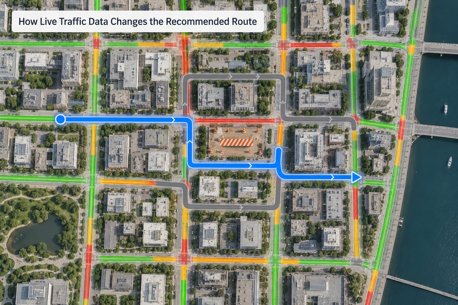
A static map is wrong the moment a lorry stops in a lane. Live traffic fixes that by replacing the free-flow speed on each road segment with a current estimate, which turns the graph into a time-dependent network where the same edge costs more at 5pm than at 11am.
Three inputs feed those estimates. Observed speeds come from phones reporting their position, which is dense on motorways and sparse on small residential streets. Probe and loop detector data is accurate but fixed in place. Predicted speeds fill the gaps, drawn from historical patterns for that segment, that weekday and that hour.
Recalculation triggers on a few concrete events: a segment’s speed drops past a threshold, an accident or closure appears in the feeds, a bus reports delay beyond its slack, a missed connection invalidates a timed transfer, or the traveler’s actual position diverges from the one the plan assumed. Good planners also re-rank continuously, not just on triggers, because a route that is three minutes worse now can be twelve minutes worse by the time you reach that stretch.
Predictions have a real edge over observation, because a segment that has not yet slowed down is the one you want to avoid early. The cost is trust: a forecast built on historical patterns is wrong exactly when the pattern changed, and you cannot tell from the map which segments are observed and which are guessed.
How Do Planners Rank Routes With Multiple Travel Modes?
Multimodal planning stops treating the trip as one graph. It runs a separate search per mode, then stitches the results together, and the stitching rules matter more than most people expect.
Transfer penalties are the core mechanic. Every mode change costs extra minutes, because changing platforms, finding a stop and boarding have friction that a straight-line time model ignores. Without a penalty, the cheapest-looking itinerary is often three buses and a walk through a district nobody planned to be in.
Waiting time is treated differently from travel time, because a wait is a certainty and a drive is a guess. Ten minutes of waiting for a bus that comes every fifteen is cheaper in practice than a predicted twelve-minute drive that regularly takes twenty-two. Frequency and reliability therefore enter the score, not just scheduled duration.
First and last mile carry the most weight for transit routes. A train journey that is 40 minutes but starts with a 25-minute walk rarely wins, because the walk cannot be shortened. A trip planner aimed at city travel optimizes the whole chain, not the middle of it, and a good one will offer a slightly slower bus that leaves from nearer your door.
Consider a cross-city trip with three plausible answers. Driving takes 35 minutes door to door but includes parking and traffic risk, a bus takes 55 minutes with one wait of seven minutes, and a tram plus a walk takes 48 minutes with a transfer at a street-level stop. A planner weighting transfers heavily returns the bus, because the tram’s transfer risk sits on a single unsignalized junction. A planner weighting total time returns the car. Same city, same hour, two defensible answers, and the difference lives entirely in the penalty values.
How Does a Trip Planner Account for Transfers and Schedules?
Timetabled routing is a lookup problem layered on top of the search. The planner does not just find fast roads, it finds a sequence of scheduled trips where each one is actually catchable by the next.
Transfer feasibility means checking real arrival against real departure, on the actual stop rather than the stop’s centroid. That requires a buffer, because a bus running two minutes early can cost you a connection and twenty extra minutes of waiting. Planners typically set a minimum connection time of a few minutes and add slack for late-running services, and the size of that buffer is one of the main reasons two apps disagree.
Service frequency changes the arithmetic too. A route on a train every ten minutes and a route on one every ninety look identical in a schedule screenshot and behave nothing alike when something goes wrong. High-frequency lines absorb delay, which is why a route using more vehicles often beats a route using fewer, especially with a tight connection at the end.
Trip planners also model the things that make a transfer fail in the field: platform changes, a bus that does not wait for a delayed train, a lift out of service at a station, and the last departure that will get you home. Those edge cases are where the difference between a theoretical connection and a usable one shows up.
Why Do Two Planners Suggest Different Routes?
When two apps disagree, one of them is not lying. The differences are almost always in the data or the weights rather than in the mathematics, which is broadly settled.
Different map data. One app may have a new pedestrian bridge, a revised one-way street or a cycle lane recorded a month before the other. OpenStreetMap-based planners and commercial map providers disagree most often on minor paths, which is exactly where a walking route diverges.
Different update times. Traffic feeds, timetables and construction notices are pushed at different cadences. The app with the freshest closures will confidently send you past a barrier the other one still sees as open.
Different weight settings. One planner optimizes for time, another for tolls or distance, and a third lets you choose. Two apps can return genuinely best routes for two different objectives and both be right.
Different transfer assumptions. Minimum connection times, whether a walking transfer is allowed at all, and how much slack a late service gets all change the ranking of transit routes more than most people expect.
Different constraints. Step-free routing, ferries only, avoid unpaved roads, daylight hours, and vehicle dimensions all prune edges the other planner never considered.
Different forecasts. Congestion prediction is the least standardized layer, so two apps can weight the same road differently at 4pm on a Friday. Developers building planners report this as the hardest complaint to debug, since a route that looks obviously worse is often just a different cost model.
What Makes a Route Recommendation Useful in a Smart City?
The shortest path is a solved problem. What a city actually needs from its routing layer is a recommendation a resident can trust and act on, and that raises the bar well past speed.
Reliability beats speed as a goal once trips get complicated. Showing a range instead of a single arrival time, and flagging a connection with only four minutes of slack, tells a passenger something true. A confident-looking estimate that fails twice a week destroys more trust than a slightly worse route.
Accessibility data has to reach the algorithm, not just the map. Step-free access, elevator working status, slope and surface quality are what decide whether a recommended route is usable for a wheelchair user, a parent with a stroller, or someone moving a heavy load. Where that information is missing, the honest move is to say so rather than to guess flatly.
Air quality and noise let a city bias routing toward quieter, cleaner corridors at a small time cost, which turns a mobility tool into a public health tool. Curb and kerb data does the same for freight and accessibility, since where a vehicle stops determines whether a wheelchair user, a cyclist or a resident can pass. Equity matters here too: a planner that optimizes only for average travel time will systematically route around low-income areas where speeds are slower and street networks are more fragmented.
Two things limit all of this. Privacy, because real-time vehicle traces can reveal where people work and live, and explainability, because a recommendation nobody understands is a recommendation nobody follows. Showing the trade-off that produced a route, three minutes saved versus one extra transfer, converts an opaque score into a decision a person can make. Cities that publish their weights and their data quality get better feedback than cities that publish only a map.
Frequently Asked Questions
What algorithm is most commonly used to plan a trip?
For a single origin and destination, a shortest-path method such as Dijkstra or A* does the work, usually on a pre-processed graph built with contraction hierarchies. Once you add multiple stops, the planner switches to a routing heuristic: nearest neighbour for a quick first answer, then 2-opt, genetic algorithms, simulated annealing or ant colony optimization to improve it. No single algorithm wins everywhere, which is why production engines combine several.
How does a trip planner use real-time traffic data?
It replaces the free-flow speed on each road segment with a current estimate drawn from phone probe speeds, loop detectors and historical prediction for that hour and weekday. Those updated costs make the graph time-dependent, so the same road is expensive during rush hour and cheap at midnight. When a segment’s speed drops past a threshold, the planner re-runs the search and reroutes around the congestion.
Does the shortest route always have the shortest travel time?
No. Distance and time are different cost functions, and they disagree constantly in real cities. A shorter road may be single-lane, signalized, school-zoned and slower, while a longer expressway can save twenty minutes. The same applies to cost: the shortest path often burns more fuel and costs more in tolls. A planner that weights time will beat a distance-based one on arrival, and the right choice depends on your trip.
How do transit planners find routes with transfers?
Transit routing is a timetable lookup layered on a shortest-path search. The planner builds the network of walk, bus and rail legs, assigns each leg a cost that includes travel time, walking effort, a transfer penalty and expected waiting based on service frequency, then searches for the cheapest chain. Each connection is checked against a minimum connection time with added slack, so a planned transfer is one you can realistically make rather than one that only works on paper.
Why might two trip planners recommend different routes?
Most often because they optimize different objectives or read different data. One may weight time, another tolls or distance. Their map versions, construction notices, traffic update times and minimum connection times can also differ, as can their forecasts for the same road at the same hour. Accessibility constraints such as step-free access, ferry-only routes or vehicle limits prune edges one planner never sees. Both results can be correct for the question each one was asked.
How often should a route be recalculated while traveling?
Recalculate on events rather than on a fixed timer: a sudden speed drop ahead, a closure appearing in the feed, a missed connection, or your actual position diverging from what the plan assumed. A well-built planner also re-ranks continuously, because a route that is three minutes worse now can be much worse by the time you reach that stretch. What to avoid is constant rerouting on marginal changes, which makes the ETA and the directions unstable.
Conclusion: Start With the Travel Objective
Ranking two route recommendations, check four things rather than distance: total time, number of transfers, cost, and how much slack each connection has. A route that is six minutes longer with one bus instead of three is usually the better one, and no amount of algorithmic cleverness will tell you that unless you look at the transfers.
Underneath, every planner does the same thing. It builds a weighted graph, searches it for the cheapest path, sequences the stops with a heuristic, filters the result against real-world constraints, and re-weights the edges when conditions change. Knowing that sequence is what turns a surprising detour into an explanation you can check.