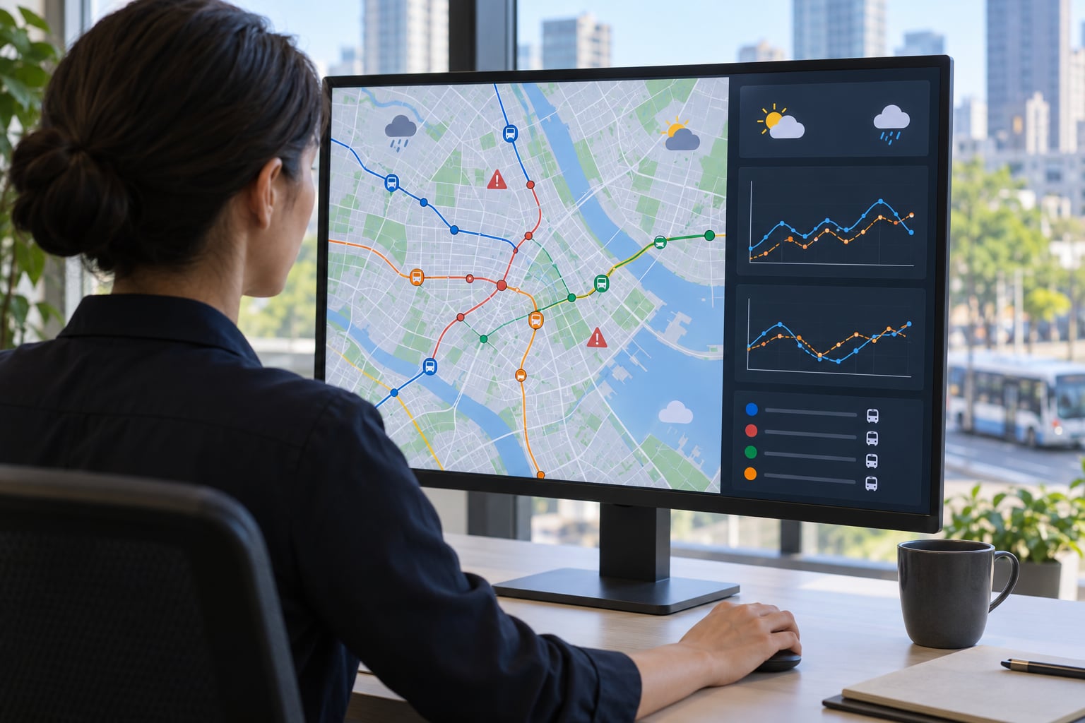
Machine learning predicts transit delays by training a model on years of past trips — scheduled times, vehicle GPS traces, weather and incident reports — until it learns the patterns that make a bus or train run late. At the moment of a trip, the model reads current conditions and returns a number: how many minutes late this vehicle is likely to arrive.
That number sounds simpler than the machinery behind it. In practice a delay model is a small pipeline that joins six or seven data sources, turns raw vehicle positions into dozens of derived signals, and produces a forecast that somebody has to decide whether to trust.
This guide walks through that pipeline end to end. It is written for transit analysts, developers and city mobility teams who need the mechanism, not for riders waiting on a platform.
Table of Contents
- What Does Machine Learning Predict in Transit?
- Static forecast or live arrival estimate
- What a good prediction actually commits to
- How machine learning predicts transit delays
- How machine learning predicts transit delays in six steps
- Why one year of history can be worse than one quarter
- What Data Does a Transit Delay Model Need?
- GTFS and GTFS-Realtime are the backbone
- Features that carry most of the signal
- Which Machine Learning Models Are Used?
- Why most agencies end up running two models
- How Accurate Must Transit Delay Predictions Be?
- Why a time-based split changes every number you quote
- How Can Transit Agencies Use Delay Predictions?
- How the prediction reaches the rider
- What Are the Main Challenges and Limitations?
- Where models quietly go wrong
- How Do You Build a Reliable Transit Delay Predictor?
- A realistic open tooling stack
- Frequently Asked Questions
- Can machine learning predict unexpected transit delays?
- How much historical data is needed to predict bus delays?
- Is a machine learning model better than using the published schedule?
- What is the difference between predicting arrival time and detecting a delay?
- How do transit agencies handle delays caused by accidents or extreme weather?
- Can riders receive accurate predictions without sharing personal data?
What Does Machine Learning Predict in Transit?
Machine learning delay prediction is the practice of training a model on historical schedule and vehicle-position data so it can estimate, before or during a trip, how many minutes late the vehicle is likely to be. It turns a stream of past observations into a forward-looking number.
In practice, transit agencies forecast a few different things:
- Arrival delay at the next stop. The most common output. Minutes late, per stop, refreshed every 30 to 60 seconds.
- End-of-trip delay. How late a bus or train will finish its run, which matters for crew and vehicle planning.
- On-time probability. Not a single number but a share: this trip has an 82 percent chance of landing inside the agency’s on-time threshold.
- Bunching risk. The chance that a vehicle will arrive close behind the one ahead of it.
- Cascade exposure. Which downstream trips and segments are about to inherit this delay.
Static forecast or live arrival estimate
Two different questions get blurred together. A static forecast answers “how late will trip 214 be when it reaches downtown at 5:15 pm tomorrow,” and it is generated minutes or hours ahead from schedules, calendars and weather. A live estimate answers “when does the next bus arrive,” and it is recalculated against current vehicle positions and traffic.
Most deployments run both, and they deserve separate models. A live estimate is mostly signal processing; a static forecast is where historical patterns and day-type features do most of the work.
What a good prediction actually commits to
A useful model commits to a horizon and a resolution. Predictions 5 minutes out on one route are a different problem from predictions 90 minutes out across a 300-bus network. Teams that skip this step end up reporting one accuracy figure for four different tasks, which tells nobody anything.
How machine learning predicts transit delays
The whole process fits in six steps. Each one is unglamorous, and skipping any of them is where projects go wrong.
How machine learning predicts transit delays in six steps
1. Define the target. Decide what you are predicting and at what granularity. “Minutes late at arrival, per trip, at each of 40 scheduled time points” is a workable target. “Bus performance” is not.
2. Collect and align data. Pull historical schedules, vehicle position traces, weather observations, incident and construction records. Join them on trip ID and timestamp so each row describes one vehicle at one moment on one route.
3. Engineer features. Derive the signals a human would use: recent delay on this route, schedule slack, day of week, holiday flag, peak-hour indicator, segment length, weather at departure, how long the vehicle dwelled at the last stop. Raw coordinates rarely help; derived schedule adherence does.
4. Train the model. Fit a regression model that maps features to minutes of delay. Gradient-boosted trees are the usual first choice because they handle mixed feature types, missing values and non-linear interactions without much tuning.
5. Validate on time. Hold out the most recent weeks as the test set, not a random sample. A random split leaks the future into the training set and inflates accuracy by a wide margin.
6. Serve the forecast. Score every new trip on a schedule, push the results into a GTFS-Realtime feed or an operations dashboard, and monitor the error over time rather than trusting the training score.
Why one year of history can be worse than one quarter
Network patterns drift. A route reconfigured last spring, a construction project closed a block, a new signal priority changed travel times on the arterial. A model trained on a year of data blends all of those regimes together and averages them into a prediction that fits none of them well.
One published project on the topic reported this directly and trained on a single quarter instead. Most teams land in the same place: weigh recent observations more heavily, or retrain monthly.
What Data Does a Transit Delay Model Need?
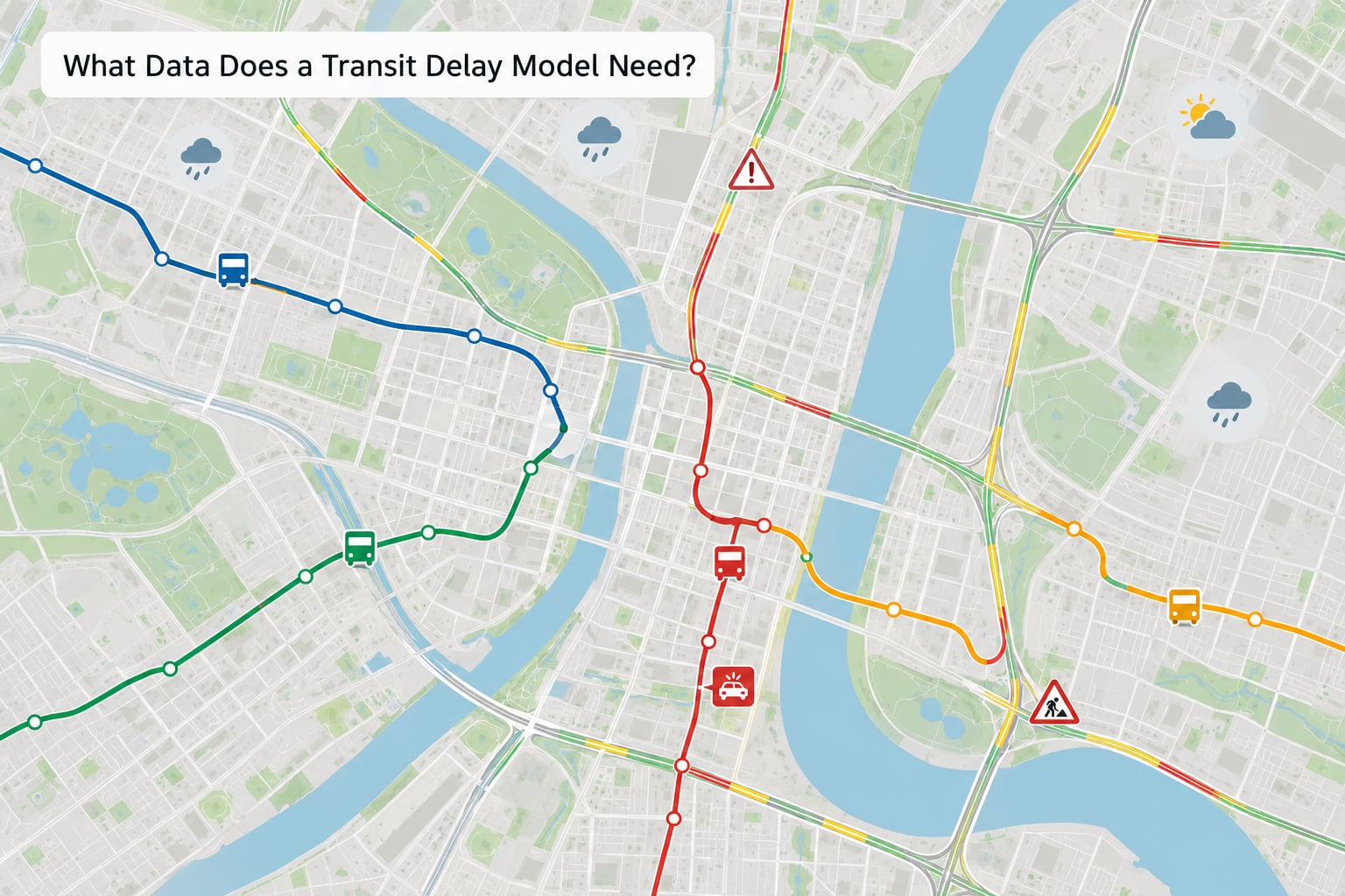
Every delay model is really a join across several feeds. GTFS is the transit backbone: a published static schedule of routes, stops and planned arrivals. GTFS-Realtime adds the live layer — vehicle positions, trip updates and service alerts. Most agencies publish both, and both are free to download.
| Data source | What it contributes to a delay prediction |
|---|---|
| GTFS static schedule | Planned departure and arrival times, route shape, stop sequence, scheduled headways |
| GTFS-Realtime vehicle positions | Where each vehicle actually is right now, and the delay it has accumulated so far |
| Historical AVL and GPS traces | Months of past runs — the training labels that make delay a learnable quantity |
| Road and traffic conditions | Congestion level on segments a route shares with general traffic |
| Weather observations | Rain, snow, ice and temperature at departure time, which change speed and boarding time |
| Incident and construction feeds | Crashes, lane closures and roadworks, often the biggest single explanation for a large delay |
| Passenger load and fare tap data | Boardings per trip, a driver for dwell time and crowding on high-ridership routes |
| Service records | Vehicle ID or tail number history — chronic late performers and mechanical flags travel with the bus |
GTFS and GTFS-Realtime are the backbone
Two terms do most of the work in any conversation about transit data. GTFS is the timetable in a machine-readable form: routes, stops, trip patterns, scheduled times. GTFS-Realtime is the live overlay, usually a feed of positions and trip updates that refreshes every 30 to 60 seconds.
For delay prediction, GTFS gives you the plan and GTFS-Realtime gives you the truth about how far the plan has slipped. Agencies publish these to open data portals, so a small city or a student project can start with real data before any vendor contract is signed.
Features that carry most of the signal
Across published work, a handful of feature groups do most of the predicting. Recent delay history on the same route at the same time of day is the strongest single signal. Day type and holiday flags matter because a Saturday timetable behaves nothing like a Tuesday one. Schedule slack — the gap built into the timetable — tells you whether a small delay gets absorbed or spreads.
Weather and incidents add the non-recurrent part. And in network models, the tail number matters more than people expect: the same bus that ran late yesterday tends to run late today, so vehicle identity is worth carrying as a feature.
Which Machine Learning Models Are Used?
Four families cover almost all real deployments. They differ in what they eat, what they are good at, and how much work they cost to maintain.
| Model family | Typical inputs | Strengths | Weaknesses | When to use it |
|---|---|---|---|---|
| Linear and ridge regression | Tabular delay features | Fast, transparent, a useful baseline | Misses interaction effects | As the benchmark every other model must beat |
| Tree ensembles (random forest, gradient boosting) | Tabular delay features | Strong on mixed data, handles missing values, fast to retrain | Noisy on long time sequences | Default choice for single-route and per-trip prediction |
| Sequence models (LSTM, GRU) | Ordered history of positions and delays | Catches temporal patterns across a whole trip | Needs lots of data and careful tuning | Long routes with rich, consistent vehicle traces |
| Graph and spatiotemporal models | Network of stops and links with time-varying state | Models cascade and network-wide effects | Heaviest to build, sensitive to sparse graphs | Multi-route networks where delay propagates |
Why most agencies end up running two models
Recurrent delay and incident delay are different problems wearing the same clothes. Recurrent delay follows the calendar: it is heavy at 8 am, light on Sunday, and repeats at the same stop every Tuesday. A model can learn that from ordinary history.
Non-recurrent delay comes from a crash, a signal failure or a snow event. Those examples are rare, so there are few labelled cases to learn from, and they arrive with almost no warning. Most teams train one model for normal operation and a second, separate one for incidents, or fall back to a rule plus a wide confidence interval when no incident model is available.
It is also worth saying plainly that a complex architecture does not automatically win. The most recent public write-up on graph-based delay modelling found that adding temporal layers did not beat a simpler static graph model on sparse data. Complexity has to earn its place.
How Accurate Must Transit Delay Predictions Be?
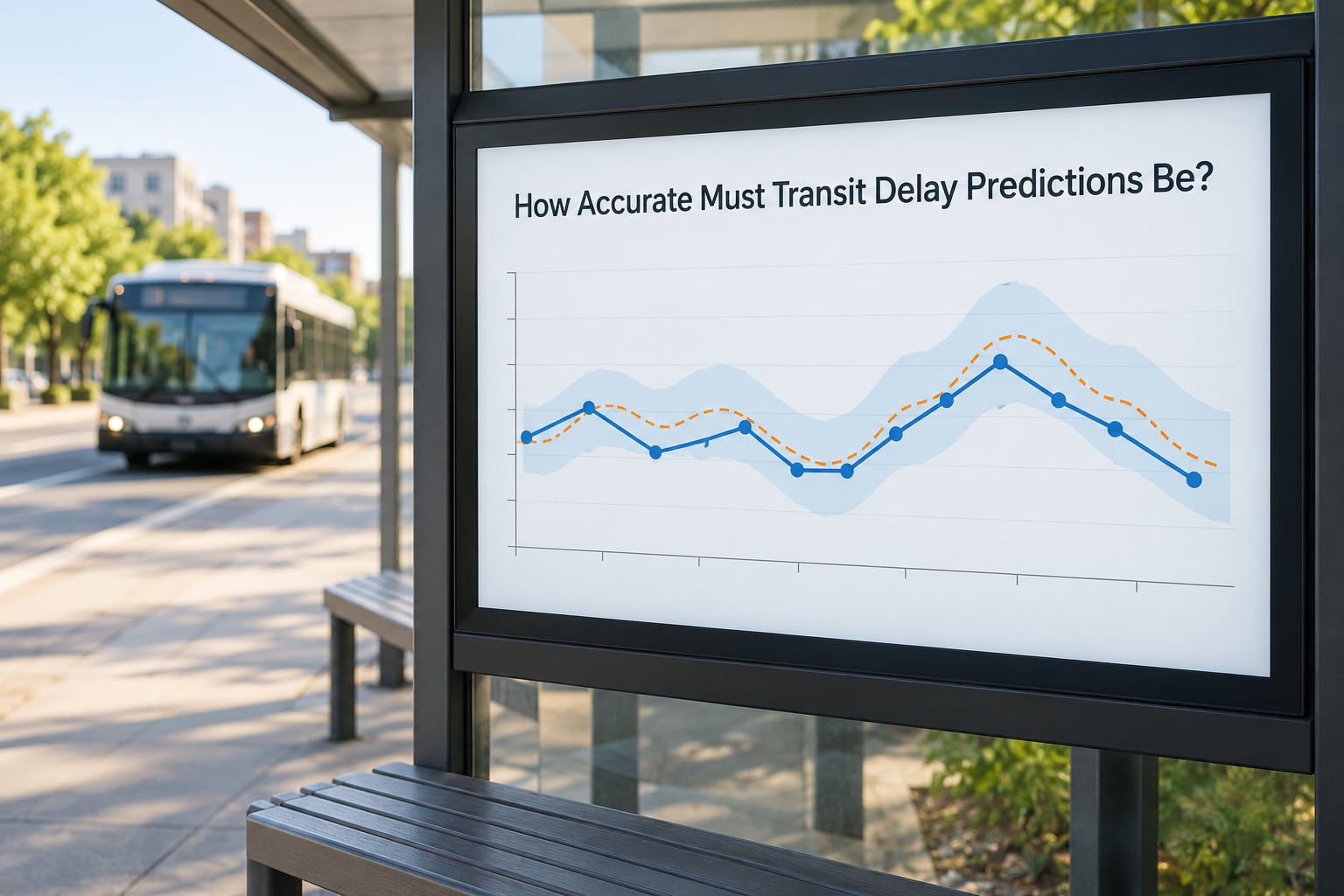
Transit delay prediction accuracy is usually reported with three numbers: mean absolute error, root mean squared error, and the share of predictions landing within an acceptable band. Which one matters depends on who the prediction is for.
| Metric | What it measures | Who should care most |
|---|---|---|
| MAE (mean absolute error) | Average size of the miss in minutes, with every error weighted equally | Anyone reporting a headline figure to operations |
| RMSE (root mean squared error) | Same idea but penalises large misses far more heavily | Teams where a badly wrong prediction is expensive |
| Within-tolerance accuracy | Share of predictions inside a band such as plus or minus 5 minutes | Rider-facing information, where “on time” is the meaningful claim |
| On-time performance lift | Change in delivered on-time performance when predictions drove holding or dispatch decisions | Agency leadership and boards |
Published numbers vary enormously with horizon, route and city, which is why any figure quoted without its methodology deserves suspicion. One widely cited road-network travel-time project reported that 87 percent of its predictions landed within plus or minus 15 seconds and 76 percent within plus or minus 10 seconds — a five-minute horizon on a highway corridor, with no incident prediction in scope. Bus systems running 20-minute routes in mixed traffic are a different problem entirely, and tolerance bands of 3 to 5 minutes are the realistic target there.
Why a time-based split changes every number you quote
Splitting your data randomly leaks information. The same bus, the same driver and the same weather pattern appear in both training and test sets, and the model effectively memorises them. Accuracy looks great and means nothing.
Split by time instead: train on months 1 through 9, validate on month 10, test on months 11 and 12. The number will be worse, and it will be the number that survives contact with a live system. This was one of the clearest findings in the recent public work on the problem, and it held by a large margin.
There is a second trap here. If you build features from actual arrival times for trips that have not happened yet, you have leaked the label into the features. Always use only information available at prediction time, which for a static forecast means the schedule, the calendar and the forecast weather — nothing else.
How Can Transit Agencies Use Delay Predictions?
The prediction is only worth the decision it improves. Agencies put forecasts to work in six common places.
Passenger information. Real-time arrival estimates replace the frozen scheduled time in apps and station displays. This is the highest-visibility use and the one riders judge most harshly.
Bus holding and headway management. When the model sees bunching forming — two vehicles about to arrive together — a controller can hold the lead vehicle briefly to restore even spacing. Done well, this improves reliability more than any schedule change.
Dispatch reassignment. When a vehicle is projected to be badly late, the controller can send a spare vehicle or swap the operator, while there is still time to act.
Service planning. Aggregated forecasts over months reveal which segments chronically fail in the afternoon peak, which is the evidence behind a timetable rewrite.
Fleet and crew planning. End-of-trip delay projections feed block and shift planning, so vehicles are not assigned a run they cannot finish.
Reliability reporting. Predicted on-time performance gives a forward-looking number to board meetings instead of last month’s failure report.
How the prediction reaches the rider
The serving path is the part most write-ups skip, and it decides whether the whole project matters. A model that retrains nightly but scores trips every six hours is worse than no model at all.
Typical cadence: vehicle positions arrive every 30 to 60 seconds, a scoring job runs on that stream or on a short timer, and the result is written into a GTFS-Realtime trip update that apps and displays already consume. The heavy work — retraining, feature recomputation, threshold tuning — runs on a separate, slower schedule, usually nightly.
Confidence has to travel with the number too. Publishing a range rather than a point estimate, and widening the range when recent error on that route is high, keeps riders from treating a shaky forecast as gospel.
What Are the Main Challenges and Limitations?
Every delay model has failure modes, and the honest ones are worth listing because they are what practitioners actually complain about.
Incidents are rare. A city might see a few dozen significant disruptions a year against hundreds of thousands of trips. There is simply not enough labelled data, which is why most incident models are either rules or anomaly detectors with a wide error band.
Concept drift is the default. Routes change, construction comes and goes, timetables get rewritten. A model degrades quietly unless someone watches its live error and triggers retraining.
Offline accuracy collapses online. The most common report from practitioners working on demand and crowding forecasting is that a model which performed well in batch falls apart once it meets a live serving loop. Freshness of features is usually the culprit.
Data is fragmented and inconsistent. Small agencies often lack reliable vehicle position feeds altogether, and some data stays paywalled. Google Transit feeds and national open data portals help, but coverage varies a lot by region.
Label leakage in schedule-only features. Building features from data that only exists after the trip completes makes results look great and fail immediately in production.
Where models quietly go wrong
One specific bug deserves naming: post-disruption over-prediction. Once a blockage clears, models trained heavily on disruption periods keep predicting delay, because the recent history still looks like a blockage. Operators then see ETAs that are 8 minutes late when the bus is running on time, and they stop trusting the output. Retraining on a rolling window and explicitly modelling recovery is the fix.
There is also the equity problem. Predictive information delivered only through a smartphone app helps riders who already have good connectivity and a data plan. Riders who rely on transit because they cannot drive are often the least well served by predictive ETA, which is one reason agencies still keep physical displays and posted timetables.
How Do You Build a Reliable Transit Delay Predictor?
Here is the path I would take on a real project, roughly in order.
1. Start with the schedule as the baseline. Before any model, measure how accurate the published timetable already is. If the schedule is off by six minutes at rush hour, no model needs to be shipped until someone fixes that.
2. Get clean data and check it hourly. Load GTFS and GTFS-Realtime, join on trip ID, and write basic quality checks: missing trips, position updates that arrive out of order, impossible speed jumps, duplicated runs. Most projects lose their first month here, and that is the correct amount of time to lose.
3. Build features from schedule adherence. Recent delay per route per time block, schedule slack, day type, holiday flags, peak indicator, dwell time at the previous stop, rolling averages over the last 5 and 20 trips.
4. Train a simple model first. Ridge regression, then random forest, then gradient boosting. Compare all three. If the boosted model does not beat the linear one by a clear margin on a time-based split, ship the linear one.
5. Split by time and report the honest number. Train on older data, test on the most recent weeks. Report MAE, RMSE and within-tolerance accuracy together, with the tolerance band stated.
6. Add a separate incident path. Do not try to fold crashes and closures into the main model. Use rules or an anomaly detector that widens the prediction band when disruption feeds go live.
7. Ship behind a confidence threshold. Serve predictions continuously, but only surface them in rider apps when the model’s recent error on that route is inside an acceptable range.
8. Monitor and retrain on a schedule. Track live error by route and time of day. Retrain weekly or monthly, and trigger an immediate retrain after a route change or a schedule rewrite.
A realistic open tooling stack
A small agency or city team can do this without a big contract: GTFS and GTFS-Realtime as inputs, Postgres or DuckDB for storage, Python with pandas and scikit-learn or XGBoost for training, a scheduled job for scoring, and a GTFS-Realtime output feed that existing rider apps already read. A graph or sequence model is worth adding only after the tree ensemble is running in production and you know exactly what it gets wrong.
Frequently Asked Questions
Can machine learning predict unexpected transit delays?
Partly, and it is honest to be cautious here. Sudden events like crashes, signal failures or medical emergencies arrive with almost no warning and are too rare to train on directly. Most agencies run a separate incident path made of rules and anomaly detection that widens the prediction range rather than guessing a single number. Recurrent delays, the large majority of late trips, are predicted far more reliably.
How much historical data is needed to predict bus delays?
Enough to cover every seasonal and calendar regime you care about, usually six to twelve months of vehicle position traces. You also need more than you expect in good weeks, because weekends, holidays and school terms all behave differently. Teams often find that one recent quarter outperforms a full year, because older runs reflect routes and construction patterns that no longer exist.
Is a machine learning model better than using the published schedule?
On most routes, yes, but measure it first. Before building anything, compute how far the published timetable runs from actual arrivals. That schedule is your baseline, and a model only earns its maintenance cost if it beats it on a time-based test split. On routes with generous slack and light traffic, the timetable is genuinely hard to beat, and many agencies use the model only where it wins.
What is the difference between predicting arrival time and detecting a delay?
Detection compares actual arrival to scheduled arrival and reports a number after the fact or in the moment. It answers whether the trip is late right now. Prediction estimates arrival before the vehicle reaches the stop, which requires modelling traffic, weather and history. Detection is comparatively easy and needs no machine learning; prediction is the harder problem and is what this guide describes.
How do transit agencies handle delays caused by accidents or extreme weather?
They feed those events in as separate signals rather than expecting the base model to absorb them. Incident and construction feeds are joined to the trip on time and location, and when one is active the system either switches to an incident model or widens the confidence interval. In snow, the practical lever is often a day-type flag combined with the forecast, since every run on that day is slow.
Can riders receive accurate predictions without sharing personal data?
Yes, and this is the normal case. Delay forecasts come from schedules, vehicle positions, weather and public incident feeds, none of which are tied to an individual rider. Trip and fare tap data can sharpen demand and dwell-time estimates, but they are aggregated before use. The systems that do collect personal information are payment and ticketing, which are separate from the prediction pipeline.
Start with the data you already have. Download your GTFS feed and your agency’s GTFS-Realtime positions, measure how far the schedule actually runs, and see where the losses concentrate. That one afternoon of work tells you whether a delay model is worth building, and it tells you which routes it should cover first.