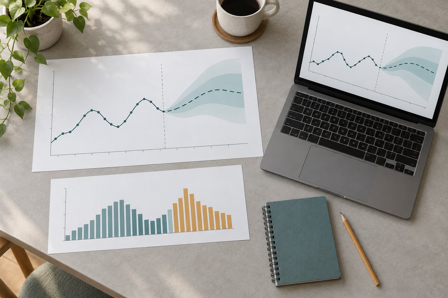
Time series forecasting works by finding repeating patterns in historical, time-stamped data and projecting those patterns forward. That is the whole idea. Everything else — the model names, the software, the error metrics — is machinery built around that single move.
This guide is written for people who have never opened a forecasting library. No linear algebra, and only as much statistics as you need to make a sensible decision. We will use small city-data examples throughout, because a bus timetable or an hourly electricity reading teaches the concepts faster than stock prices do.
Table of Contents
- What Is Time Series Forecasting?
- How Time Series Forecasting Works for Beginners
- What Data Does a Time Series Model Need?
- How to Prepare Time Series Data
- How Time Series Models Learn Patterns
- Trend
- Seasonality
- Cyclical variation
- Noise
- Autocorrelation and smoothing
- Which Forecasting Method Should Beginners Use?
- A Beginner Forecasting Example
- How time series forecasting works for beginners, end to end
- How Do You Measure Forecast Accuracy?
- Common Time Series Forecasting Mistakes
- Frequently Asked Questions
- How much historical data do I need for time series forecasting?
- Do I need machine learning to make time series forecasts?
- How do I forecast when the data has missing values?
- What is the difference between a trend and seasonality in time series data?
- Can external variables improve a time series forecast?
- How uncertain should a beginner’s forecast be?
- Conclusion
What Is Time Series Forecasting?
Time series forecasting is the practice of predicting what a measured quantity will do next by studying how it behaved in the past. A time series is simply a list of observations, each stamped with a time, where the order of the observations carries meaning. A city air-quality sensor logging PM2.5 every hour is a time series. So is daily transit ridership, monthly electricity load, or the number of bike-share trips leaving a dock.
That last part is what separates forecasting from ordinary prediction. If you surveyed 500 residents about their commute, the order of those answers tells you nothing. Shuffle them and nothing breaks. With a time series, shuffling destroys the signal: this morning’s reading is strongly related to last night’s, and Monday tells you something about Tuesday that Sunday does not.
The practical consequence is that forecasting methods carry a built-in assumption — the past is a decent guide to the near future. When that assumption fails, you get concept drift, which is simply the world changing underneath a model that was trained on the old version of it.
How Time Series Forecasting Works for Beginners
A forecasting project follows a fairly fixed path, and you can get through a first one without much math. Here are the seven steps, in the order that saves beginners the most time.
- Define the target and the horizon. Write down exactly what you are predicting, how far ahead, and how often. “Next Tuesday’s 8am corridor bus load” is a forecastable question. “How busy will transit be?” is not.
- Inspect the data first. Plot it. Look for trend, weekly or yearly seasonality, gaps, spikes and flat stretches. Most beginner mistakes are visible in a line plot before any model is involved.
- Prepare and clean. Fix timestamps, fill or flag missing observations, decide what to do with outliers, and add date-based features such as hour-of-day and day-of-week.
- Build a naive baseline. Forecast tomorrow with today’s value, or this week with the same week last year. This is your floor, and no model earns a place until it beats it.
- Split by time, not by chance. Train on the older data, test on the newer data. Randomly shuffling rows leaks future information backwards and inflates your score.
- Fit a model and compare it to the baseline. Start simple. Add complexity only when the validation numbers say you have earned it.
- Forecast forward and state the uncertainty. Produce values for the forecast horizon along with a range, because a single number implies a confidence the data rarely supports.
Steps one and four get skipped most often, and both are cheap. A clearly scoped question and a naive baseline take under an hour and save days of model tuning that was never necessary.
What Data Does a Time Series Model Need?
Every forecast needs a time column, a target column with a numeric value, and enough rows to cover the seasonal cycle you care about. Everything else is optional help. A typical open-city dataset for hourly foot traffic might look like this.
| Column | Type | Role |
|---|---|---|
| timestamp | Datetime | The time axis, regular intervals preferred |
| sensor_id | Text | Groups rows when several sites report separately |
| footfall_count | Integer | The target you predict |
| hour_of_day | 0-23 | Derived feature, daily seasonality |
| day_of_week | Mon-Sun | Derived feature, weekly seasonality |
| temp_c | Number | External variable, optional |
| is_holiday | 0 or 1 | External variable, optional |
Note the word regular. Most models assume evenly spaced observations, so an hour that vanished because a gateway dropped offline is a real gap you have to handle. Rows that describe several sensors at once also need care: mixing them into one series creates a sawtooth pattern that is an artefact of your data collection, not a real cycle.
The train-versus-test split is the other non-negotiable. For hourly data, train on everything up to a cut-off point and test on what came after, the same way the future will arrive.
How to Prepare Time Series Data
Preparation is unglamorous and it decides your results. Run through this list before modelling anything.
- Check the time axis. Sort chronologically, confirm a fixed interval, and confirm there are no duplicated timestamps. Daylight saving shifts and leap days create gaps that look like anomalies if you do not handle them deliberately.
- Look at missing values. Decide per gap: drop the day, interpolate a short gap from neighbours, or add a missing-value flag and let the model know the measurement was absent. Silently replacing a gap with zero creates a fake trough.
- Investigate outliers before deleting them. A reading of 9000 passengers in an hour may be a real event, not a broken sensor. For civic data, the spike often is the story.
- Add date features. Hour, day of week, month, week of year, and flags for holidays and school terms. These cheap columns often beat a fancier model on their own.
- Scale only when a model needs it. Tree-based and classical statistical models do not care about units. Models built on distance or gradient descent do.
- Guard against leakage. Any feature computed using information unavailable at prediction time is cheating. Centering or imputing with the whole dataset, rather than the training portion, leaks the future into the past.
If you only take one habit from this section, make it plotting the series before anything else. A five-minute line chart catches most data problems that would otherwise be blamed on the model.
How Time Series Models Learn Patterns
Most models decompose a series into a few moving parts, then learn each part separately. Four components explain the vast majority of what you will see.
Trend
Trend is the slow direction of travel. For a growing city, hourly electricity load drifts upward year over year even after you remove the daily cycle. A model that captures trend but not seasonality will be accurate in the morning and badly wrong at 6pm.
Seasonality
Seasonality repeats on a known calendar: daily rush hours, weekday versus weekend, summer versus winter, term-time versus holidays. It has a fixed length you can name, which is exactly what separates it from the next component.
Cyclical variation
Cycles have no fixed period. A heatwave pushes electricity demand up for six days and then it relaxes; a roadworks scheme reroutes traffic for four months and then ends. Forecasting a cycle means judging that the swing is temporary.
Noise
Noise is what remains after the other three are removed. It is the residual, and you cannot forecast it. What a good model does is shrink its influence rather than chase it, which is the entire logic behind smoothing.
Autocorrelation and smoothing
Autocorrelation simply means near values are related: today’s reading carries information about yesterday’s. Inspecting how correlation decays across lags tells you which lag lengths matter. Smoothing is the practical response — averaging over a recent window, so a single strange reading moves the forecast a little rather than a lot.
Consider hourly grid load on a weekday. Level sits near 400 kW overnight, the morning peak reaches roughly 900, and a level spike from one broken meter should not move tomorrow’s curve. A smoothed model responds to the shape while ignoring the spike.
Which Forecasting Method Should Beginners Use?
Start at the top of this table and move down only when the row above it stops being good enough. Most beginner projects never leave the first three rows, and that is a perfectly respectable outcome.
| Method | Best for | What it needs | Difficulty |
|---|---|---|---|
| Naive forecast | The baseline every model must beat | Nothing but the last value | Trivial |
| Moving average | Short, noisy series; smoothing jagged data | A window length | Trivial |
| Seasonal naive | Strong daily or weekly repeat patterns | One full seasonal cycle of history | Trivial |
| Exponential smoothing | Trend plus seasonality with clean data | Enough cycles to fit smoothing levels | Low |
| Linear regression with date features | Adding external drivers such as weather | Well-chosen features | Low |
| ARIMA or SARIMA | Longer history with clear autocorrelation | Stationary series, usually differenced | Medium |
| Machine learning regression | Many related series and rich external features | Substantially more data and care | Medium to high |
| Deep learning | Very large datasets, long horizons, many series | Compute and real expertise | High |
ARIMA stands for autoregressive, integrated and moving average — past values predicting the future, differencing to remove trend, and smoothing over recent errors. SARIMA adds explicit seasonal terms. If you remember one thing about ARIMA, it is that it needs a stationary series, which usually means differencing first to remove the trend.
Community recommendations on forecasting forums lean heavily toward Hyndman’s Forecasting: Principles and Practice, a free online text, over paying for a course. That matches what practitioners actually do.
A Beginner Forecasting Example
How time series forecasting works for beginners, end to end
Suppose a city publishes hourly footfall counts from one sensor in the shopping district, and the transport team wants next week’s figures to schedule extra trams. The full workflow looks like this.
Scope it. Target: hourly count. Horizon: 7 days ahead. Refit weekly, since new data arrives daily.
Prepare. Sort by timestamp, confirm a strict hourly interval, and flag the two hours lost to a gateway outage rather than filling them with zeros. Add hour-of-day and day-of-week columns.
Baseline. The seasonal naive rule — use the same hour from the previous week — is the honest first attempt, because shopping footfall is strongly weekly. If that already gets within about 12% on average, the bar for anything cleverer is high.
Model. An exponential smoothing model with weekly seasonality fitted on the previous six weeks of history. No tuning parameters, no deep network.
Forecast. A typical weekly output looks like this.
| Period | Predicted count | Expected range |
|---|---|---|
| Mon 08:00 | 840 | 760 to 930 |
| Mon 18:00 | 1420 | 1290 to 1580 |
| Sat 14:00 | 1760 | 1590 to 1960 |
| Sun 14:00 | 980 | 870 to 1100 |
Read it honestly. The tram planner cares about the Monday evening peak, not the average, so that peak needs an added safety margin rather than a midpoint. The Saturday and Sunday difference is the model earning its keep, because seasonal naive with a weekly rule would already capture it. A widening range later in the horizon is honest, not a bug: uncertainty compounds the further out you project.
How Do You Measure Forecast Accuracy?
Accuracy is measured by comparing predicted values with what actually happened on data the model never saw. Three metrics cover almost all beginner needs.
| Metric | What it measures | Use it when |
|---|---|---|
| MAE | Average size of the miss in the target’s own units | You want an interpretable number for planners |
| RMSE | Average miss, punishing large errors heavily | Big errors are far worse than small ones |
| MAPE | Average miss as a percentage | Comparing series of different sizes |
A contrast makes this concrete. On a test week, a strong model averaged about 95 misses (MAE 95, MAPE around 11%). A weak model averaged about 310 misses (MAE 310, MAPE 34%). Reporting the weaker model in percentage terms alone would hide that its worst days were off by more than 700 people, which matters a great deal if you are running tram capacity on the number.
One trap: MAPE breaks when actual values are near or equal to zero. An air-quality series with calm nights at zero PM2.5 will produce meaningless percentages. Use MAE there, or sMAPE, and say which one you used.
Validation should also respect time. Rolling or expanding-window cross-validation — train up to a date, test on the next block, slide forward — gives a fairer picture than one split, especially for short horizons.
Common Time Series Forecasting Mistakes
These six account for most failed first forecasts, and each has a straightforward fix.
- Randomly shuffling the data before splitting. Fix: split by time. Train on older rows, test on newer rows, always.
- Using future information in a feature. A “final revised ridership figure” column already contains the answer. Fix: audit every feature for what was knowable at prediction time.
- Ignoring seasonality. Fix: plot the series grouped by hour or weekday before fitting anything.
- Skipping the baseline. Fix: always report naive performance beside your model, including on the test period.
- Fitting a model with too little data for its complexity. A seasonal model needs at least two full cycles. Fix: simplify the model or gather more history.
- Reporting a single number as certainty. Fix: publish a prediction interval and refresh the forecast as new data lands.
Frequently Asked Questions
How much historical data do I need for time series forecasting?
Enough to cover the seasonal cycles you want the model to learn. For hourly data with a daily and weekly pattern, aim for six to twelve weeks. For monthly data with an annual cycle you need two to three full years. Very short series can still be forecast with naive methods, but they cannot support complex models, and more data is usually better than a cleverer model.
Do I need machine learning to make time series forecasts?
No. Naive forecasts, moving averages, seasonal naive and exponential smoothing are statistical methods, not machine learning, and they handle a surprising share of real civic and operational series. Learn those first, measure them honestly, and reach for machine learning only when you have external drivers, many related series, or a baseline you have genuinely beaten.
How do I forecast when the data has missing values?
Never replace a gap with zero unless zero is truly what happened. Short gaps can be interpolated from neighbours, while longer gaps are better left missing with a flag column so the model knows the measurement was absent. Before either fix, check whether the gap is a sensor problem, a deliberate change in collection, or a real event worth reporting on its own.
What is the difference between a trend and seasonality in time series data?
Trend is the slow underlying direction of the series, such as gradually rising electricity demand as a city grows. Seasonarity repeats on a fixed, known calendar cycle: hourly, weekly, monthly or annual. Trend has no fixed period, seasonality always does, and that difference is what tells you whether to use a plain model or one with seasonal terms.
Can external variables improve a time series forecast?
Often yes. Weather, holidays, events, road closures or policy changes add information the historical series cannot express on its own. Add them as features, but only ones known at prediction time, and check on a time-based test split that they genuinely help. A long weather forecast is itself uncertain, so treat it as a range rather than a fixed input.
How uncertain should a beginner’s forecast be?
Report a range, not a point. Prediction intervals widen as the forecast horizon grows, and a wider band is a signal of less information rather than a failure. Say which model produced the interval and over what data, and reissue the forecast whenever new observations arrive so decision-makers see how accurate the last one was.
Conclusion
Time series forecasting rewards discipline more than cleverness. If you are starting now, do these five things in order: write down the target and forecast horizon, plot the series and read off its trend and seasonality, build a seasonal naive baseline, validate with a time-ordered split, and only then add a model. If it does not beat the baseline on a fair test, ship the baseline.
Once a simple model is working, the interesting part begins: adding external drivers, comparing short and long horizons, and being honest about how wide the prediction interval should be. That is where a useful forecast starts to inform real decisions.